Serveur © IRCAM - CENTRE POMPIDOU 1996-2005.
Tous droits réservés pour tous pays. All rights reserved.

Prediction of the Spatial Informations for the Control of Room Acoustics Auralization

Federico Cruz-Barney et Olivier Warusfel

AES: Convention of the Audio Engineering Society, New York City, Etats Unis, Septembre 1997
Copyright © Audio Engineering Society 1997

Abstract

This paper presents some results on a study aiming at accessing the spatial information needed for the recreation of realistic binaural impressions of enclosed spaces from echograms simulated by a room acoustics predictive software developed at IRCAM. After a brief description of the software and of the general principle of auralization in computer models, a simple formulation to obtain the binaural criteria IACC using the predictive software is explained and some attempts to validate it are made.

Introduction

In order to recreate realistic auralizations of the acoustics of enclosed spaces, one usually convolves an anechoic signal (music, speech,...) with binaural impulses obtained either from measurements with a dummy head in a real room or a scaled model, or by simulations with a computer model. When the simulated outputs of a predictive software are instead given in the form of energy-time curves (ETC), as with the present software, convolution is no longer possible and the necessary spatial informations for the binaural reproduction of the entire soundfield is not directly accessible. This paper presents a method aiming at compensating for the lack of spatial information of the ETC by the estimation of an associated mean incidence vector per temporal segment at each one of the receiving positions. The calculated mean incidence vectors are then used to control the spatial cues of the different time sections.
As an example, a simple method to calculate the interaural cross-correlation coefficient IACC from our computer software using this principle is proposed in order to have access to binaural auralizations.
After a brief description of the main characteristics of the predictive software developed at IRCAM, the basic principle of the auralization process that we use is explained, followed by an explanation of the method proposed. Finally, an attempt to validate it is done using a data base gathered from a measurement campaign undertaken at IRCAM's Espace de Projection.

Description of the room acoustics predictive software

The room acoustics laboratory at IRCAM has developed a room acoustics predictive software [1] that combines various physical models of sound propagation to estimate the energy-time curves at different receiver locations. These models include plane wave propagation with specular reflections, diffraction and diffuse reflections. The combination of these methods is derived from preliminary studies showing their complementarity when estimating different criteria linked to the acoustical quality of a hall. Figure 1 shows a schematic description of the models involved in the prediction process, briefly explained in the following paragraphs.

Diffraction model (step 1). In the presence of an orchestra pit or loggia in an Opera house, a geometrical masking of the direct sound will occur for certain parts of the audience. In such a case, the diffusion and the specular reflection model would reflect the energy back into the incident half space, considering that complete masking occurs, instead of a resulting diffracted wave. The perceptual importance of the direct sound has led to the introduction of a diffraction model to account for this sort of situation.
Model of plane wave propagation and specular reflections (step 1). The plane wave propagation is simulated by an algorithm combining an image source model up to second order reflections with a cone method for the prediction of higher orders of reflections.
Diffuse propagation model (step 2). In order to take into account the non-specular character of reflections, the preceeding models are coupled to a method based on the hypothesis of ideally diffuse reflections (Lambert's law). The combination of the specular and the diffuse models is managed for every reflection according to a diffusion coefficient depending on the nature of the walls (or facets). The fraction of energy not specularly reflected nor absorbed is propagated between the room boundaries according to a transfer matrix, computed during a preliminary process (step 0 in figure 1), and that describes the time and space discretisation of Kuttruff's integral equation [2].
Late energy propagation (step 3). After a transition time (Tt), the cone method and the direct diffusion processes are stopped and the residual energies present on the boundaries are used for the calculation of the late energy distribution. Assuming an exponential decay, the amplification of this residue is calculated for each boundary and the corresponding energy contributions are checked on each receiver location (figure 2). Hence the late energy distribution will depend on the following parameters:
1. distribution of the residual intensity when the cone tracing method is stopped;
2. amplification of this residue during the exponential decay;
3. geometrical coupling of the receivers with each surface.

This particular method gives access to the distribution of the late reverberant field, which under some circumstances may not be homogeneous, as is the case with balcony overhangs.
The reverberation time may be obtained from procedures described in [1][3].
The usual energy-based parameters which characterize the acoustical quality are then derived by subdividing the energy-time curves into temporal segments or ``pre-criteria'' (see table 1).

Auralization in computer models

When dealing with the computer modelling of binaural impulse responses (BIR), the early and late parts are often obtained by separate procedures [4][5]. The early part is generally calculated by inverse Fourier transform of the transfer functions of the minimum-phase equivalent filters characterising the different phenomena encountered by each sound ray along its propagation path for a given source/receiver couple. They include the source directivity, the air absorption, wall reflections and diffraction from the listeners head, torso and ears (as measured by the Head related Transfer Functions, HRFT). The later part of the BIRs can be synthesised using various statistical approaches. One of them consists in substituting the late part of the response with white noise filtered according to the mean absorption of room boundaries, to the air absorption and to the diffused field response of the source and the receiver [5]. Another approach consists in creating the late part by a simplified process associated to a shoebox shaped hall with the same mean free path, absorption factor and surface area as the actual hall [4]. A simulation of the auralization inside the model is then obtained by convolution of the entire binaural response with an anechoic signal. Its performances when compared to the simulated space will depend on the different physical models used to characterize the sound propagation, transducers characteristics, halls geometry and the materials data base. However, the results obtained are only valid for a single source/receiver couple and so the BIRs have to be recalculated for every source or receiver position and orientation. Another inconvenience comes from the fact that the procedure is based on a binaural encoding of spatial cues, thus auralizations will only be valid for an individual reproduction on headphones (binaural mode) or two loudspeakers via a cross-talk cancellation filtering matrix (transaural mode). This limitation can be partially overcome when encoding the acoustic field at a receiving position with the 4-channel Ambisonic ``B format'', which is equivalent to the coincident association of an omnidirectional microphone and three orthogonal bidirectional microphones [6]. In this case, Ambisonic decoders can accommodate various multichannel loudspeaker layouts of typically four to eight loudspeakers and allow a post processing to simulate orientation effects of the receiver [7].

An alternative approach for the auralization consists in describing the acoustical quality perceived at each receiver location by a set of parameters instead of an impulse response, and to synthesize the room effect according to these parameters. In the present case this synthesis is performed by the Spatialisateur, a virtual acoustics processing software developed at IRCAM and Espaces Nouveaux [8]. The Spatialisateur synthesizes, in real time, a generic room effect which is controlled by a set of parameters issued from research carried out at ENST and IRCAM [8][9]. This generic room effect is based on a simplified temporal distribution of the energy, consisting in four time sections (figure 3). After synthesis of the time distribution, the Spatialisateur controls the spatial informations associated to the different time sections: localisation control for the direct sound and early reflections (OD + R1), and control of the IACC for the binaural reproduction of the cluster and the late reverberation (R2 + R3).
The energy of the time sections may be computed from the ETCs generated by the room acoustics predictive software. On the contrary, the spatial informations associated to each section are not directly accessible. Hence, the control of the spatial parameters of the Spatialisateur requires some additional information given by the computer model and described below.

Direct sound. The spatial information related to the direct sound is of special importance since it will govern the localisation of the source. However, in case of direct sound masking, linked to diffraction by room edges or to directivity characteristics of the source, this first contribution might be substituted with the first reflection. The spatial information provided to the Spatialisateur is simply the direction of incidence of the sound path associated to this first contribution. The Spatialisateur will use this directional information to synthesise the localisation according to the chosen reproduction setup.
Early reflections. Concerning the early reflections, a direction of incidence can be associated to each one of the reflections synthesised by the Spatialisateur, as for the direct contribution. However, some studies [10] suggest that auditory perception may not be sensible to the fine structure of the early reflections distribution. Hence, it may be envisionned to simplify the spatial description of this time section, which can lead to save signal processing cost, especially when using binaural coding. A simplification is proposed in [11]. It consists in keeping the interaural gain and delay differences for each reflection and to filter the whole early reflections section by the use of a common filter. This common filter can be calculated from the HRTFs associated with the reflections included in that time section and weighted by their respective energies.
late reverberation. In order to characterize the perceived spatial effect associated to the late reverberant energy, the computer model should provide an estimation of the interaural cross-correlation coefficient IACC [12][13][14].

One of the advantages of this parametrical approach is to provide a description of the auditory scene independently from the reproduction configuration. Whereas a characterization based on impulse responses will be more constraining, for it is linked to a specific encoding format of the spatial information. More generally, such a parametrical approach allows post-processing operations. For example, the head-tracking, used to compensate for the movements of the listener during the auralization, may be easily implemented since it consists in a correction of the directionnal parameter send to the Spatialisateur. Hence it does not involve additional processing cost.

Estimation of the spatial cues

In order to estimate the spatial cues associated to the time sections of the ETC, the description of the spatial distribution of reflections is synthesised in the form of simple indices. For this purpose, a mean incidence vector is calculated. The norm of this vector will provide the information about the diffuseness of the soundfield at a particular time section and its orientation will translate a lateralization effect eventually perceived by a listener. These informations will be used to estimate an IACC associated to a particular time segment.

In the following paragraphs the calculation of the mean incidence vector is explained along with the description of a method proposed by Nakajima et al.[15] for the estimation of the IACC and an alternative simple method which relates with possible IACC values for given temporal sections of the ETC.

Calculation of the mean incidence vector V

For every one of the energy contributions (specular or diffused) to a specific receiver, the mean incidence is calculated and weighted according to the amount of energy carried by the contribution as well as to the receivers directivity. A vector

of components (

) as viewed from each receivers coordinate system is then constructed, where

corresponds to the receiver pointing direction,

to the lateral direction and

to the upward/downward direction. Once this vector is known, its three components will provide the vertical and horizontal (

) angles of incidence for a particular time section. The IACC can be estimated from the vectors norm

and from an equivalent angle measured from the receivers median plane, a lateralization angle

of the soundfield as seen from the receiver, where

. This approximation is justified since we can consider the head as being almost symmetrical, so the IACC is mainly determined from the reflection angle measured from the median plane [15].

Nakajima's method for the estimation of IACC

For the estimation of the IACC within the context of computer simulations, a proposed procedure is inspired from a method developed by Nakajima et al.[15], where a simple equation to calculate the IACC was derived. The method consists on the recreation of the interaural cross-correlation function CCF by the superposition of the elementary CCF cumulated for each reflection and for a specific frequency band. The normalized value of the resulting CCF for N discrete and incoherent reflections at both ears of a human or dummy head can be expressed in the following terms:

where

is the time delay of sound signals between both ears, and ranges from -1ms to +1ms to include the maximum interaural delay.

is the pressure amplitude of the nth reflection relative to the direct sound.

is the CCF of the signals for the nth reflection and its associated lateralization angle

and

are autocorrelation values ACF at

=0 (arrival time of the direct sound) of the signals at the left and right ears, for the nth reflection and associated lateralization angle

. The interaural cross-correlation coefficient IACC corresponds to the maximum absolute value of the function.
The independent bandpass-filtered components of the CCF of centre frequency

, are calculated by the following equation:

where

is the CCF per octave band ( m ) of the signals for the nth reflection, B is the effective bandwidth of the noise;

is the crosspower of mth bandpass filtered source signals at both ears normalized by that of

(frontal incidence). The value of

indicates the delay at the maximum of the cross-correlation function, which depends on

Estimation of IACC from the mean incidence vector V

Since for a given sound signal, the IACC will be a function of the directions as well as of the amplitudes of sound reflections arriving at a receiver, an approximated method is now proposed to relate the vectors

to possible IACC values.
The maximum possible IACC value per octave band for a given angle of incidence is obtained in free field. For that particular case, the norm of the mean incident vector

will equal unity. In an ideally diffuse sound field, the cross-correlation between two omnidirectional microphones is related to the ratio sin(kr)/kr, r being the distance between both receivers. At low frequencies, the receivers will be closer to each other relative to the wavelength, so high correlations are to be expected. While

will reach a value very close to zero at all frequencies, IACC will vary depending on the octave band.

The mean incidence vectors obtained in the precedent section for given temporal segments and for specific frequency bands are then related with a simple equation to possible IACC values ranging from supposed minimum diffuse field IACC()_D up to a maximum established by a set of free field measurements which will depend on the lateralization angle . So, each estimated IACC() per time segment from simulations, IACC(,t) will be a function of the following variables: the free field IACC(,), the diffuse field IACC()_D and :

Validation of the method from a measurements data base

A measurement campaign has been undertaken at IRCAM's Espace de projection, a variable acoustics rectangular room by means of an adaptable volume ( 1800m³ - 3800m³) and rotating panels covering all walls and ceiling [1]. The data base gathered from this campaign has been used to validate the method for the estimation of the IACC using the room acoustics predictive software developed at IRCAM. In this section, the measurement campaign is explained and the results obtained are shown along with the validation procedure.

Measurement campaign

The impulse response measurements were carried out using an MLS based measurement system. A dodecahedron loudspeaker was used as the sound source which was placed on the axis of the room at some distance to the back wall. Two Shoeps electrostatic microphones of the colette series, with a multidirectional capsule model MK6 in its omnidirectional configuration and attached to a home made dummy head were used as receivers (figure 4). Four receiving positions and four room configurations with a fixed volume were tested, giving a total of sixteen source/receiver combinations. The room configurations were the following:

AA: All of the acoustic panels of the room (ceiling + walls) in the absorbent position.
RR: All of the acoustic panels of the room (ceiling + walls) in the reflecting position.
AR: All of the front half of the room (ceiling + walls) absorbent, the back half reflecting.
RA: All of the front half of the room (ceiling + walls) reflecting, the back half absorbent.

IACC values for the 3 octave bands centred at 250Hz, 1KHz and 4KHz were derived from the impulse responses measured at both ears of the dummy head selecting the maximum absolute value of the interaural cross-correlation function (CCF_t()) within the integration limits t₁ and t₂:

where l and r represent the left and right ears respectively, and

the time shift, ranging from +1ms to -1ms to include the maximum interaural delay.

For the validation of the method, simulations on the computer model of the Espace de projection were performed for all the acoustical configurations and according to the same spatial disposition, directivity and orientation of the transducers.
Comparisons between the estimated and measured IACC for the time range from [0 - 80ms], IACC₈₀ and the three octave bands are presented and discussed in the next paragraphs.

Results and discussion

As a first approach to the validation procedure, some preliminary results from comparisons at the 250Hz, 1KHz and 4KHz octave bands between measured and estimated IACC₈₀ are presented.

In order to have an idea on the objective differences between the configurations tested, table 2 shows the measured and simulated reverberation time (RT) variability. The measured (RT_s presented are the mean values of the left and right ears at all of the receiving positions for a given configuration. Eventhough the RT change from the most absorbent to the most reflective configuration is quite important, as seen in table 2, the IACC₈₀ range between configurations is relatively small, for the geometry of the room remained unchanged during the measurement campaign. As a result, the robustness of the validation is somehow limited.

Table 3 illustrates the overall statistics of the measurement campaign. From the mean difference between measurements and the computation model we see that there is a tendency to underestimate IACC₈₀ for all three frequency bands, a tendency very much accentuated at receiver position R2, which is probably related to a particular reflection pattern associated to this receiver position.
Although the Standard Deviation (STD) statistics show that estimated values variate less than the measured ones, the inter-receiver and inter-room configuration variations are well predicted, as seen from the Mean Absolute Error results (after correction of the global difference), and from the Correlation Coefficients. Figure 5 shows inter-receiver variation results for the three frequency bands tested and for room configuration RR. An example of inter-room configurations estimation is presented in figure 6. Results for configurations AR and RA and for two receivers, R2 facing the first half of the room and close to the source, and R4, far from the source and in the back half of the room (see figure 4) are given. For room configuration RA, low correlation values are expected for receiver R2, since for the time segment studied strong reflections will hit the receiver from a relatively wide solid angle, whereas for R4, reflections coming from a smaller solid angle will predominate, because it is surrounded by absorptive surfaces. In this case then, higher IACC₈₀ are expected. The estimated IACC₈₀ follow this trend quite well, as for the opposite situation (configuration AR) where correlation values at receiver R2 will be higher than for the precedent configuration and will diminish at receiver R4.

The observed differences found concerning the smaller estimated variations in relation to the measured ones and the global underestimated IACC₈₀ , may be related to the approximations inherent to the estimation method in the one hand, and to the fact that, because the are periodical functions with several maxima (their separation depending on frequency), reflections coming from different directions interfere with each other and contribute to increase the measured inter-receiver variability, on the other. Actually our method is closer to an approximation of the CCF by their envelopes, i.e. where the estimation of the IACC from the mean incident vector is equivalent to the estimation of IACC calculated from the superposition of the envelopes of the in equation 1.

Conclusions

A simple method for the calculation of the spatial cues associated to the different time sections of the simulated ETCs from our room acoustics predictive software has been presented. This method includes the estimation of the IACC in order to have access to binaural auralizations. For the validation of the method, IACC estimations in three frequency bands have been compared to a data base gathered from a measurement campaign undertaken at IRCAM's Espace de projection.

For the measurement sample tested, results are coherent. Both inter-receiver and inter-room configuration variations are well predicted. The global differences found concerning the estimated variability, as given by the STD, and the error estimation related to the measured IACC₈₀ are probably the consequence of the method approximations that do not consider periodicity.

To further validate the method and confirm this behaviour, the measurements data base has to be extended to other room shapes and sizes. Time intervals without the direct sound must be compared since the examples tested were very much influenced by the direct sound because of the receivers proximity to the sound source.

References

1: Christian Malcurt. Simulations informatiques pour predire les critères de qualification acoustique des salles. Comparaison des valeurs mesurées et calculées dans une salle à acoustique variable. PhD thesis, Université de Toulouse, 1986.
2: Heinrich Kuttruff. Room Acoustics. Elsevier Applied Science, London, 3^rd edition, 1991.
3: E.N. Gilbert. An iterative calculation of auditorium reverberation. J. Acoust. Soc. Am., 69(1):178-184, 1981.
4: Bengt-Inge Dalenback. Room acoustic prediction and auralization based on an extended image source model. PhD thesis, Chalmers University of Technology, Göteborg, Sweden, 1992.
5: Marc Emerit. Simulation binaurale de l'acoustique de salles de concert. PhD thesis, Institut National Polytechnique de Grenoble, 1995.
6: M.A. Gerzon. Ambisonics in multichannel broadcasting and video. J. Audio Eng. Soc., 33(11), 1985.
7: Jean Marc Jot. Real-time spatial processing of sounds for music, multimedia and interactive human-computer interfaces. Multimedia Systems Journal. Special issue on Audio and Multimedia, 1997.
8: Jean Marc Jot. Etude et réalisation d'un spatialisateur de sons par modèles physique et pérceptifs. PhD thesis, Ecole Nationale Supérieure des Télécommunications, 1992.
9: Jean-Pascal Jullien. Structured model for the representation and the control of room acoustical quality. In 15th Intl. Congress on Acoustics, Trondheim, Norway, pages 517-520, 1995.
10: D.R. Begault. Binaural auralization and perceptual veridicality. In Proc. 93rd Audio Eng. Soc. Convention, San Francisco, USA, preprint 3421 (M-3), 1992.
11: Jean Marc Jot, Olivier Warusfel, Eckhard Kahle and Mireille Mein. Binaural concert hall simulation in real time. In IEEE Mohonk workshop, Oct 17-20, 1993.
12: J.S. Bradley. Comparison of concert hall measurements of spatial impression. J. Acoust. Soc. Am., 96(6):3525-3535, 1994.
13: P. Damaske and Y. Ando. Interaural Crosscorrelation for Multichannel Loudspeaker Reproduction. Acustica, 27(1):232-238, 1972.
14: Takayuki Hidaka, Leo L. Beranek and Toshiyuki Okano. Interaural cross-correlation, lateral fraction, and low- and high-frequency sound levels as measures of acoustical quality in concert halls. J. Acoust. Soc. Am., 98(2):988-1007, 1995.
15: Tatsumi Nakajima, Jun Yoshida and Yoichi Ando. A simple method of calculating the interaural cross-correlation function for a sound field. J. Acoust. Soc. Am., 93(2):885-891, 1993.

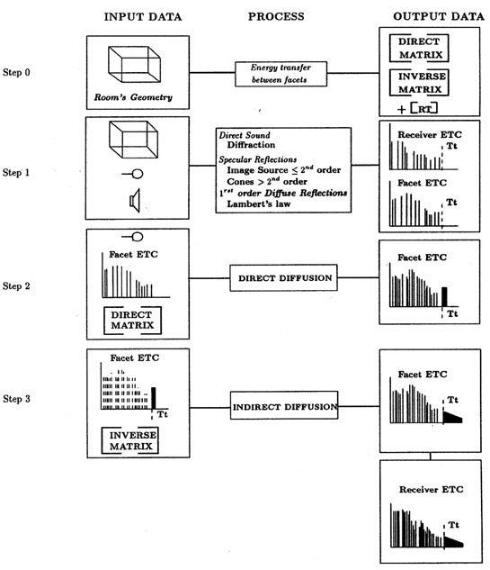
Figure 1: Schematic description of the room acoustics software. Tt stands for transition time

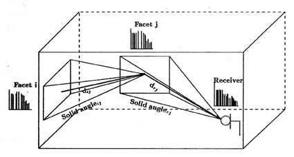
Figure 2: Diffuse energy transfer between facets and imputation to receivers

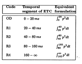
Table 1: Temporal segmentation of the energy-time curve (ETC) for the calculation of energy-based criteria. The integrals temporal limits are given in ms. The zero corresponds to the arrival time of the direct sound signal
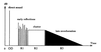
Figure 3: Generic room effect created by the Spatialisateur. Typical temporal segmentation of it is as follows: OD=[0,20]ms, R1=[20,40]ms, R2=[40, 100]ms, R3=[100, ]ms

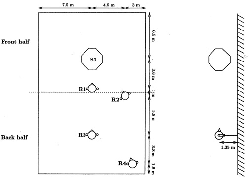
Figure 4: Configuration setup for the measurement campaign at the Espace de projection. Source (S1) and receivers (R1 - R4) placement. The ears of the dummy head correspond to the omnidirectional microphones

Centre Frequency Configuration Measured RT Simulated RT

250Hz AA 0.923 1.011

RR 2.371 2.433

AR 1.361 1.480

RA 1.492 1.606

1KHz

AA 1.258 1.207

RR 3.018 3.058

AR 1.813 1.922

RA 1.821 1.922

4KHz

AA 0.965 0.942

RR 2.138 2.239

AR 1.401 1.382

RA 1.401 1.474

Table 2: Reverberation times measured (in seconds) and simulated at the Espace de Projection. The measured RT are the mean of the four positions for the left and right ears.

Centre Frequency Measured Iacc STD Estimated Iacc STD Average difference between Sim and Meas Mean Absolute Error (after correction of global difference) Correlation Coefficient

250Hz 0.162 0.157 -0.005 0.027 0.854

1KHz 0.225 0.188 -0.064 0.051 0.801

4KHz 0.206 0.191 -0.053 0.030 0.967

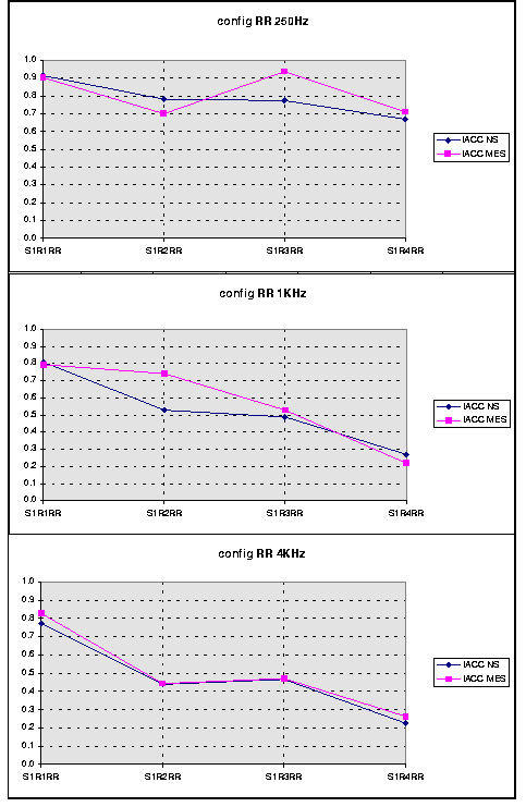
Figure 5:Comparison between measured and estimated IACC₈₀ for a single configuration, on source (S1) and four receiver positions (R1 - R4)

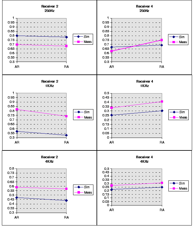
Figure 6:Comparison between measured and estimated IACC₈₀ for two receivers (R2 and R4 ), one source (S1) and two rooms configurations variability